Mathematics behind Black-Scholes options pricing

Options

A financial instrument investors use where they acquire the right to purchase or sell an underlying asset at a later date for an agreed upon price. The price at which they agree to either buy or sell the underlying asset is called the strike price. Other aspects included the time to maturity, the value ofthe stock, the risk-free rate of return, and the volatility of the underlying asset.

Black Scholes Formula

Here is a descriprion of the Black-Scholes formula:

\[\begin{equation} C(S,t) = S_0 \, N(d_1) - K e^{-rT} \, N(d_2) \label{eq:black_scholes_call} \end{equation}\] \[\begin{equation} P(S,t) = K e^{-rT}\, N(-d_2) - S_0\, N(-d_1) \label{eq:black_scholes_put} \end{equation}\] \[\begin{equation} d_1 = \frac{\ln\!\left(\frac{S_0}{K}\right) + \left(r + \frac{1}{2}\sigma^2\right)T}{\sigma\sqrt{T}} \label{eq:d1} \end{equation}\] \[\begin{equation} d_2 = d_1 - \sigma\sqrt{T} = \frac{\ln\!\left(\frac{S_0}{K}\right) + \left(r - \frac{1}{2}\sigma^2\right)T}{\sigma\sqrt{T}} \label{eq:d2} \end{equation}\]

The Greeks

Delta:

\[\begin{equation} \Delta_c = N(d_1) \label{eq:delta_call} \end{equation}\] \[\begin{equation} \Delta_p = N(d_1) - 1 \label{eq:delta_put} \end{equation}\]

Gamma (Same for call and put):

\[\begin{equation} \Gamma = \frac{N'(d_1)}{S_0 \sigma \sqrt{T}} \label{eq:gamma} \end{equation}\]

where:

\[N'(d_1) = \frac{1}{\sqrt{2\pi}} e^{-d_1^2/2}\]

Vega (Same for call and put):

\[\begin{equation} \text{Vega} = S_0 \sqrt{T}\, N'(d_1) \label{eq:vega} \end{equation}\]

Theta:

\[\begin{equation} \Theta_c = -\frac{S_0 N'(d_1)\sigma}{2\sqrt{T}} - rK e^{-rT} N(d_2) \label{eq:theta_call} \end{equation}\] \[\begin{equation} \Theta_p = -\frac{S_0 N'(d_1)\sigma}{2\sqrt{T}} + rK e^{-rT} N(-d_2) \label{eq:theta_put} \end{equation}\]

Rho:

\[\begin{equation} \rho_c = K T e^{-rT} N(d_2) \label{eq:rho_call} \end{equation}\] \[\begin{equation} \rho_p = -K T e^{-rT} N(-d_2) \label{eq:rho_put} \end{equation}\]

Further Research

Currently this version of the black-scholes model assumes that the volatility of an underlying asset is constant over the lifetime of the asset, prices can be modeled using geometric brownian motion, there is continuous rebalancing , no trading costs, and no arbitrage. These are often not possible to be replicated in the real world, especially the constant volatility and the constant risk free rate.

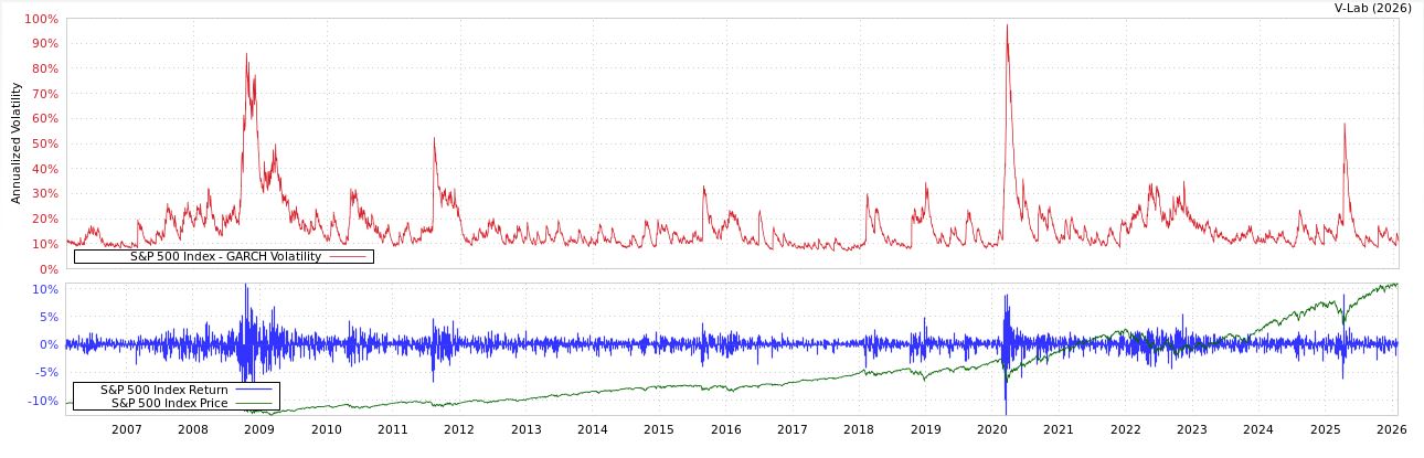
One way that we can adjust the model to fit real life is to look at the volatility of the underlying asset and adjust it from a constant to a stochastic process. This is called the Heston model. The heston model is built upon the idea that the volatility of an asset and the price of an asset are both stochastic processes and that large movements in either the price or the volaitly directly correlates with large movemetns in the other. It also follows along that volatility after large variations usually reverts to its mean or follows the principals of mean reversion.

Here is an example of the correlation between the price of the S&P 500 and it’s volatility.

… More to come